Defeating the Enemy's Artillery

INTRODUCTION

This page describes the arrangements for counter battery (CB) fire.  The enemy's field artillery normally deployed some distance back from the front line.  Therefore they were usually invisible to observation posts (OP) and forward observing officers (FOO) along the forward defence lines (FDLs). This meant they could not be engaged by ground observers in the normal way.  

CB was the general term used to attack and defeat the enemy's artillery (excluding mortars).  But before the enemy's artillery can be attacked the hostile batteries (HBs) have to be found.  Their positioning behind the FDLs meant that technical means had to be used to find HBs.  In WW1 the three most important, in order, were: air reconnaissance (visual and photo), sound-ranging and flash-spotting.  Although visual air reconnaissance does not seem to have been prominent in WW2, photo reconnaissance by Tac/R was.  Sound-ranging and flash-spotting were provided by the corps survey regiment.  Counter mortar (CM) was introduced in the last years of the war.  HBs were usually attacked in a systematic and coordinated way, often using longer range guns that weren't part of the divisional artilleries.   This was the responsibility of the CB officers (CBOs).

The CB battle in World War 2 (WW2) was nowhere near as intense as it had been in WW1.  The German artillery was relatively far smaller than in the previous war because the Luftwaffe had been given a major role in delivering firepower.  Nevertheless some 75% of British casualties in N Africa were caused by artillery and mortar fire and even in the final year of the war they caused some 61% of Red Army casualties.  While airpower worked in the early years of the war the Luftwaffe gradually lost the ability to achieve even local air superiority, but Germany lacked the resources to expand their field artillery arm so sought cheaper and simpler solutions.  

Nebelwerfers (multiple rocket launchers) were introduced in late 1942 and mortars, being cheap and simple, were also expanded.  Mortars also became widely used and British operational research found that a medium mortar was worth two MGs.  However, while these presented a negligible CB threat they were a major threat and cause of casualties to the infantry and had to be dealt with.  Despite being generally smaller than the Allies, German artillery was a significant force in Italy, often attacking Allied targets and was also heavily used in the Normandy campaign.

The Japanese artillery appears to have lacked any significant CB capability, both in guns and target acquisition, although they did engage allied artillery.  In Burma and the SW Pacific their usual method was to attack gun positions with fighting patrols, sometimes supported by artillery fire.  

TARGET ACQUISITION

As in WW1 air observation was a key means of observed fire against HBs and other targets beyond the view of ground observers.  In WW1 radio equipped aircraft were used to direct artillery fire from the first year of the war.  They also 'marked' HBs by dropping flares over them that were 'fixed' by cross observation from the ground.   In WW2 Air OPs played a useful CB role once they became available, and were later able to take useful photographs as well.  However, they were not allowed  to fly within 2000 yards of known or suspected enemy positions, which often kept them behind the FDLs.  They were also required to fly below 600 feet.  All this limited their visibility of HB deployment areas.  As in WW1 air photo reconnaissance (Tac/R) was also a major target acquisition asset.  Other RAF aircraft could report and engage ground targets, including HBs, using the Arty/R procedure, a successor to the WW1 'zone call' although it was nowhere near as useful as had been hoped before WW2.  The School of Artillery at Larkhill was the 'centre of excellence for training in air-photo reading.  These are discussed further in Other Firepower.

Cross-observation gun-spotting techniques had been taught to garrison artillery and were soon used in WW1 by the heavy and siege batteries.   It rapidly evolved into flash-spotting.  Although the British had ignored sound-ranging before WW1, they developed it quickly by inventing the low frequency microphone in 1916.  However, in early 1916 all flash-spotting and sound-ranging was put into the new Field Survey Companies (one per army, subsequently expanded to battalions) of the Royal Engineers (RE), although many of the officers and soldiers involved were artillery.  The RE also surveyed gun positions and performed cross observation amongst their many survey and map-making tasks.  After WW1 the Royal Artillery took on the target acquisition role formed its own survey companies for flash-spotting, sound-ranging and artillery survey, both regular and territorial army.  At the outbreak of WW2 these survey companies expanded into survey regiments, with one assigned to each corps.

The corps survey regiment was the primary artillery target acquisition element for CB purposes.  Initially survey regiments comprised three specialist batteries, one each for sound-ranging, flash-spotting and survey.  The regiment deployed across the corps front in defence but provided a composite sub-unit under the flash-spotting and sound-ranging battery HQs to each of the two forward divisions when operations were less static. However, in 1941 some survey regiments were re-organised into two identical composite survey batteries, each with troops for flash-spotting, sound-ranging and survey that could be assigned to the forward divisions.  This organisation, very similar to that used before WW2 when there were only survey companies RA, became standard in late 1943, and with it part of the flash-spotting battery became an observation troop in RHQ.  This undertook cross-observation tasks when air-burst ranging was used against targets out of sight to ground observers.  They also had a capability for air-photo reading and deducing target co-ordinates from air-photos.  The detailed organisation of this regiment is linked to 'Artillery Organisations'.  

The schematic layout of a survey battery assigned to a forward division is shown in Figure 1.  It shows the sound-ranging (SR), flash-spotting (FS), and survey (Svy) troops from a survey battery and a ranging (Rng) section from the regimental HQ troop.  This RHQ troop ranged friendly artillery fire onto targets by using cross observation, usually of airburst shells.  The SR troop had 2 Advanced Posts (APs), its microphone base and computing centre, the FS troop had 4 flash-spotting Posts (FSPs) and a plotting centre, and the ranging section 3 Observation Posts (OPs) and a computing centre.  The survey troop had 2 survey sections, each 3 pairs of surveyors and a computing centre.  The FS and SR troops would have direct communications to the Assistant Counter-Battery Officer (ACBO) and his section assigned to the division from the corps CB staff, where battery HQ was usually collocated, and the ACBOs had wireless directly to the corps CBO.

Figure 1 - Schematic of a Composite Survey Battery and RHQ Ranging Section in a Divisional Area

By early 1944 German mortars were becoming a significant problem and in Italy dedicated resources were introduced to deal with them.  After D-Day the German mortars took an increasingly significant toll of British infantry and the counter-mortar (CM) battle became increasingly important.  This led, in late 1944, to divisional counter-mortar batteries being formed, equipped with CM radars and new sound-ranging equipment.

FLASH-SPOTTING

The essence of flash-spotting to locate HBs was to get accurate cross-observation of muzzle flashes from at least three different positions, the flashes being either directly observed muzzle flashes or 'sky flashes'.  The real trick was to ensure that the widely separated observers were all looking at the same flash.  Flash-spotting troops were organised into an observation section of flash-spotting posts (FSP) that reported their observed bearings of muzzle flashes to their troop HQ.  This HQ provided the plotting centre. which controlled the FSPs and determined HB locations by plotting the bearings they reported, and had an intelligence task of collating their reports.  Flash-spotting became harder with increasing German use of flashless propellants from mid-war (although there was more smoke), longer range guns deploying further back also made it difficult as did the practice of deploying guns behind a ridge to mask their muzzle flash.   However, in the final months of the war German use of flashless propellants grew less and flash-spotting success increased correspondingly.  

The deployment of the FSPs depended on the terrain in the divisional area.  The posts needed height so they could see well into enemy territory.  From Tobruk onwards (including El Alamein) they sometimes used locally produced and later pre-fabricated towers to gain height and therefore visibility.  There were two types of flash-spotting 'base' (line of FSPs).  A long base  was usually 3,000 - 10,000 yards long, but could be up to 15,000.  A short base was a single post with a subsidiary position a few hundred yards away.  Accurate HB locations required observation bearings from three FSPs, and the troop had four FS parties.  The short base produced a single bearing and distance.  The FSPs also reported any other enemy activity that they observed and undertook crater and fragment analysis of hostile fire, from which bearings to the HB and the calibre of the guns could be found.  Even when it was not possible to obtain bearings to an HB from two or more FSPs a single bearing was still useful if it was to an already known battery because it signified that the battery was still in position and active.

Flash spotting was basically a night time activity, while in daylight reporting enemy activity was predominant.  However, flashless propellants produced more smoke and could reveal the gun by forming a smoke ring visible in the right conditions and muzzle flashes could be seen out to some 10,000 yards.  Gun flashes last about 1/20^th of a second and at night are visible out to about 30,000 yards in European conditions.  There are three types: directly visible muzzle flashes,  indirect flashes where the muzzle flash is invisible because the gun is behind a crest but lights up moisture in the air, and sky flashes where the cloud base is illuminated by the muzzle flash.  

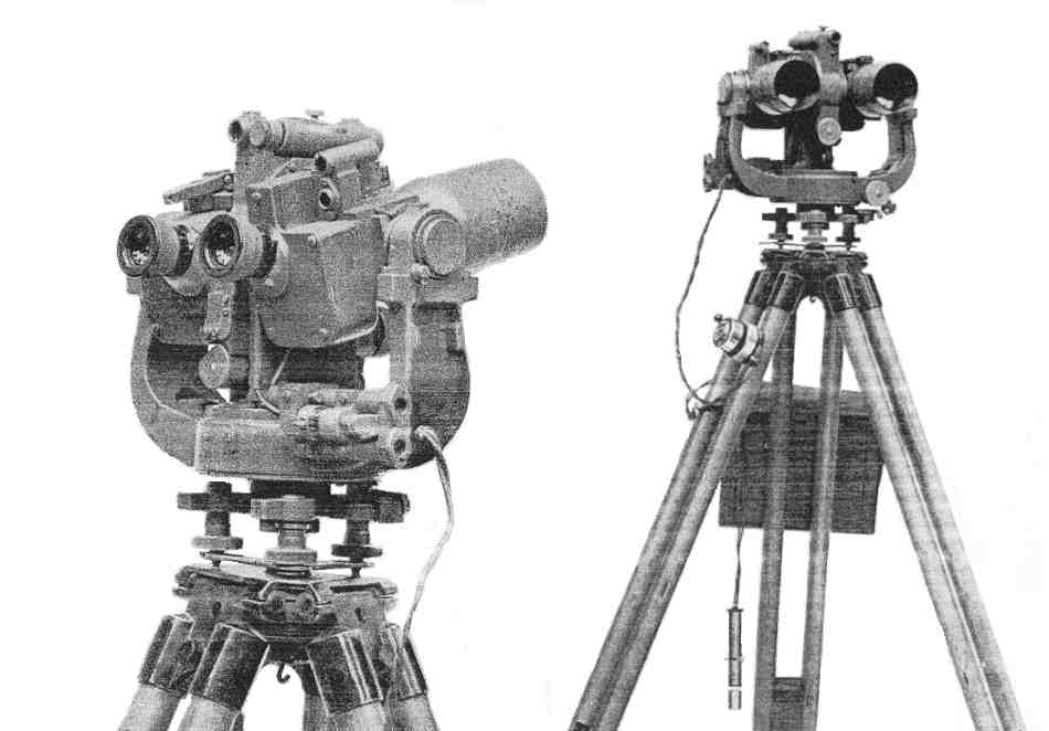
The basic equipment of a FSP was Instrument, Flash-spotting, No 4, Mk 1, shown below.  Later Mks were developed and issued during the war, by 1944 the Mk 3 was in service.  This instrument was a tripod-mounted binocular device with a bearing scale.  Posts were also equipped with more conventional instruments including a tripod-mounted high power spotting telescope that provided several magnifications up to ×30.  Communications could be by line or radio, the latter obviously far quicker to deploy.   Mk 1 instrument had a field of view of some 15°, wider than other less specialised instruments but still relatively narrow.

Figure 2 - Instrument, Flash-spotting, No 4, Mk 1

During WW1 the 'flash & buzzer switchboard' that had been developed, this enabled FSP to signal flashes as they observed them.  Each FSP transmitted a 'buzz' that was a different tone that could be heard by the others, which enabled the observers to identify the same source of flashes.  The switchboard at the plotting centre had light and buzzer displays that responded to signals from the FSPs' 'flash keys', when they flashed together then it meant that the FSPs were observing the same HB firing flashes.  They could also switch off the FSPs' buzzers to check that the FSPs really were seeing the same flashes and not echoing the buzzer of the lead FSP that initiated the observation.  However, this device seems to have been abandoned in the late 1930's.

In WW2 the FSPs and the plotting centre were connected together using telephones (D Mk 3 and later FS, Mk 1).  When a FSP detected a HB firing the observing soldier immediately reported the bearing directly to the plotting centre.  At the centre that FSP was designated the lead, the bearing plotted on the concentration board, and observation bearings were ordered to the other FSPs.  The FSPs then aligned their instruments as ordered.  When the lead FSP reported the next flash the FSPs that saw it reported their bearings, the plotting centre plotted these and changed the observation bearings for FSP that had not seen the flash.  This continued until each FSP could report a sufficiently accurate bearing to the same HB.  When observing, FSPs didn't try to centre their instrument on the flash, they used the graticule angles for measurement, applied these to their ordered bearing and reported the result.  

The concentration board in the plotting centre was gridded with each FSP position marked.  Also marked were a bearing arc for each FSP.  Generally observation bearings were plotted with fine strings and not drawn.  The concentration board was quick; more accurate locations could be found using the quadrant board.  This was gridded the same as the concentration board and also marked with two accurately inscribed arcs and the centres of their circles.  A parallel ruler was used to plot bearings from each FSP.

FSPs used stop watches to measure the 'flash to bang' time, this was useful to get a quick fix on a HB to determine whether or not it was already known.

There were several different deployment modes, which traded deployment time for accuracy of results, although deployment could be progressive to get to a fully accurate base.

• The fastest and least accurate was the short base.  An FSP established a subsidiary post several hundred yards away, the two were surveyed together.  Angles from both posts could produce HB locations with about a 'B' accuracy out to about 10,000 yards and took little more than an hour to be ready to observe.  An artillery board was used for plotting. Using the base distance and internal angles of the triangle, a slide rule or logarithms could  be used to trigometrically calculate the distance from a post to the target, this distance and bearing could be plotted or calculations again used to find the target location.
• A three post base, with the FSP's positions determined from the map and using wireless could be ready to observe in about 4 hours.  In could produce 'Z' accurate locations of actual muzzle flashes to about 20,000 yards and sky reflection flashes of about 'B' accuracy.
• A four post base, fully surveyed and using line communications could be ready to observe in about 12 hours.  In could produce 'W' accurate locations of actual muzzle flashes to about 20,000 yards and sky reflection flashes of about 'A' accuracy.

Standard accuracies, J - D,  for HB locations are given here, later on this page.

Although FS was the main method of visual observation of HB, it was not the only one.   All-arms were responsible for reporting hostile shelling and mortaring.  This used  ‘Shelreps’ (hostile shelling reports) and 'Moreps' for mortars.   This method was not particularly accurate for locations (the reported bearings were usually based on sound and rarely sufficiently accurate), but was useful in providing information about HB activity, particularly when the 'area shelled' was reported as well. ‘Moreps’ were of less value because hostile mortars tended to move more often.

Despite flash spotting becoming increasingly difficult with increasing use of flashless propellant in late 1944, at Geilenkirchen, a new electro-optical flash recorder was trialled.  This produced an accurate bearing to a flash.

Although primarily the task of the RHQ observation section, flash spotters also undertook observation tasks.  This included airburst ranging where a target was accurately known, typically from an air photo, but was invisible to a ground observer.  The guns fired HE with time fuzes and the angle of sight raised so that the airbursts could be observed and ranged, and when on target the angle of sight was dropped to ground level.  Precise observation was also used for calibration firings and  to accurately register points behind the enemy's front, for example a key point for a barrage.  

SOUND-RANGING

The Russians claim to have successfully used sound-ranging (SR) on a training range in 1910 and a German officer was granted a patent in 1913.  It evolved rapidly in WW1 although it appears that Germany made little use of technology and relied on aural detection.  One man listening to 2 microphones a couple of km apart and measuring the time interval with a stop-watch.  From this a bearing to a battery could be deduced, these somewhat inaccurate bearings were combined with those from other listeners, hopefully for the same battery.

Microphone sound-ranging needed two technologies, one to detect the low frequency sound (about 20 hertz) of guns firing, the other to record the signals in a measurable way.  The first needed the invention of the low frequency microphone using a heated platinum filament; the second adopted a French system using a 5 string galvanometer recording from 5 microphones.  In this the signal from the microphone caused its string to 'kick', the string's shadow being recorded on moving 35-mm film with time marks on it.  Sound-ranging used a base of several microphones connected to a 'Recorder, SR' in a plotting centre.  The signal from each microphone made its own line on the 'film' with a break when the sound arrived at the mike.   This revealed the relative times of arrival at each microphone of the sound of guns firing.  In WW2 British sound-rangers used either moving coil or hot wire linear microphones.

Film processing (developing and fixing using chemicals) was part of the Recorder, SR, Mk 1 at the beginning of WW2, Mks 3 and 4 appeared later in the war and produced traces for 6 microphones.   During WW2 a new pen recorder was  introduced, Recorder SR No 2, using electrical 'pens' to plot a trace-line on a roll of sensitive paper instead of film.  Both recorded the duration of the sound (to 1/100 second) and the strength of its pressure wave.  

Figure 3 - Output Trace from Recorder, SR, No 2
(Teledetos paper 3 inches wide driven at 15 or 5 cms/sec)

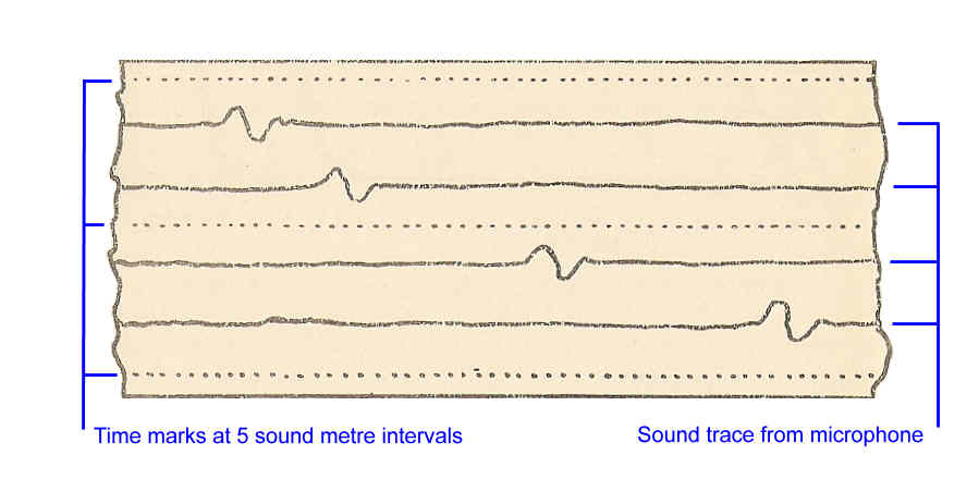
The time marks, at 5 or 10 sound metre intervals, were key to measuring the relative time of arrival of a sound at each microphone.  They were produced at the same time as the sound recording by a Strobotron driven by an oscilloscope in the recorder.  A sound metre was the time taken by sound to travel 1 metre in conditions of 50% humidity and 50° F air temperature in still air. The film or pen trace was analysed to identify the moment of firing on the trace lines for each microphone and measurements taken of the different sound arrival times.  A firing gun produces three different sets of sound waves at different frequencies:

• The gun-wave, the actual noise of the gun firing.
• The shell-wave, the noise of the shell in flight particularly when in is supersonic, this is a higher frequency sound and the need to avoid being swamped by these sound waves is what made the low frequency microphone so important.
• The burst-wave from the shell bursting.

The last could be used to range friendly fire onto an HB location.  

Figure 4 illustrates the basic set-up of a regular base using cable for communications, however radio could also be used. It wasn't practical to have the pen-recorder running continuously, therefore there had to be a way of switching it on when HBs were firing.  This required Advance Posts (AP) at least 800 metres in front of the general line of microphones and 1,000 metres if radio was being used.  

Figure 4 - Sound-ranging
Two APs were usually deployed

The AP had two important roles.  First, when he heard a HB or mortar firing and line was connected, he switched on the recorder in the sound ranging CP and switched it off when the sound wave had passed.  For this he used a Control Unit, SR (a modified field telephone) or Telephone, FS, Mk 1.  If radio was in use he instructed the CP staff to switch it on and off, this took longer hence the AP having to be further forward.   The second role was to report the direction the sound came from, this helped the CP plot the HB, including quickly checking whether it was a new or known one (this could be done by comparing traces, but was helped by knowing which traces to look at).

In addition to using the relative times of sound arrival to deduce location, the recorded sound shape of a gun-wave on the film was often distinctive for each calibre of gun, which provided important information for artillery intelligence.  It also made it difficult to spoof sound-ranging with HE explosions for deception purposes.  However, recording the gun-wave and the burst-wave enabled the time of flight  to be determined and graphs were used to find the calibre by this means as well. The problem with sound-ranging was that lots of guns firing together was liable to 'swamp' the recording.

The sound waves are affected by wind and temperature (the speed of sound varies with temperature) and so the data read from the film had to be corrected in the plotting centre.  This need for meteorological data was the main reason for each SR troop having a detachment of RAF meteorologists to provide the necessary meteorological data.

The microphone base, from 4 up to 6 microphones (depending on the type of recorder and two No 2 recorders could be used to give a base of up to 7 mikes), was about 3,000 - 5,000 metres behind the FDLs and ideally behind most of friendly field artillery positions.  A 'regular' base, where the microphones were equidistant was best from a plotting perspective because it was simplest.  A regular base could be either straight line or curved, the latter generally giving the best results.   Each microphone was paired with its neighbours and each pair was a 'sub-base'.

A straight line base would be up to about 8,000 metres, while a curved one could be as short as an arc of about 1,500 metres at a 16,000 metre radius.  The problem was fitting the base to the terrain, not too difficult in the desert but a real challenge in Burma and a fair one in Europe. Siting microphones in good listening positions was very important and the terrain could have many undesirable effects that interfered with sound. When a regular base was impossible then an irregular one had to be used.  For long range locating it was 5 - 6 microphones 1,000 - 2,000 metres apart.  It was also important to accurately 'fix' by survey the position of each microphone.  This was to a far higher level of accuracy than was necessary for gun positions.

Initially all communications between APs, plotting centre and microphones was by line, although it wasn't necessary to lay an individual line from the plotting centre to each microphone and to each AP.  One line could serve a cluster of three microphones and an AP.  However, research into the use of radio had resumed in the late 1930's and Radio Link, Sound Ranging, Mk 1  became available in 1941.  It could support up to five radio linked microphones and could be used in combination with line linked ones.  The radios used were No 11(SR) with a Sender, SR at each microphone, these each communicated on their own frequencies to their own R 105 receiver in the plotting centre.   No 11(SR) had slightly higher frequencies than the normal No 11.  Later in the war a Mk 2 radio link was introduced that used a single multi-channel receiver in the plotting centre, although it still didn't provide remote 'switch-on' for APs .  The problem with radio link was that each microphone needed men in regular attendance to keep the radios correctly tuned and to ensure charged batteries were available, see Communications.  A frequency with little interference was also important.

In the plotting centre the line or radio links were connected through a Control Unit, SR, to the Recorder, SR, No 1 which could be switched on by the AP unit when line was connected.  Once a film trace had been processed it had to be 'read' to measure the relative times of arrival of the sound wave at each microphone, corrected for met and the results converted to bearings which were plotted to find their intersection and the coordinates of this point.   

There were several methods for deducing bearings ('circle', 'graph', 'secant' and 'asymptote') using graphs or mechanical plotters, but the asymptote method gradually emerged as the preferred one.  This method deduced the bearing from the mid-point of each sub-base (2 microphones) and plotted them.  

With a regular base an Asymptote Plotter, SR, No 1 Mk 1 was used, it was constructed at 1:25,000 map scale and could be used with a map.  Irregular bases meant setting up a Board Plotting, SR, using printed celluloid time scales.  The bearing plotting process didn't use paper and pencil methods but fine strings that could be quickly laid out on the plotting board to give a ‘cats-cradle’ at the HB location.  Before WW2 a mechanical plotter had been developed but this doesn't seem to have been used during the war - the guru of sound ranging, Professor Sir Lawrence Bragg, always advised simplicity and the mechanical plotter was not simple.

Plotting wasn't normally used to range CB fire onto a HB, instead a mechanical analogue computer called a ‘comparator’ was used, it solved first-order differential equations.  This device had been introduced just before WW2 but improved and differently configured versions appeared during the war, reaching Mk 4.

The accuracy of this sound-ranging system, expressed as a Probable Error in range was approximately the square of the distance to the HB in thousands of metres.  The maximum range for locations was about 15,000 metres in an arc about 10,000 metres wide in front of the base.  A base of 6 microphones fully surveyed could produce 'Z' accuracy HB locations and took 6 - 12 hours to deploy.  Five microphones with 1,000 metre sub-bases fixed from the map gave 'B' accuracy locations but could be deployed in about 2 hours.  Of course once deployed it could be properly surveyed.

Data from sound ranging also enabled methods for estimating calibre from time of flight.  This had been used in WW1.  The data needed updating for the German equipment used in WW2.  The method was to measure the distances from a microphone to the located gun and to its shell burst, and the sound-metres on the trace between the gun firing and the shell burst.  From this the gun-target range and time of flight could be deduced.  Graphs were provided plotting curves of range against time of flight for every gun and charge combination.  From this the type of gun could usually be determined.

The problem with the older equipment was that it was not sensitive enough to detect and locate medium (8.2-cm) mortars.  However, in June-July 1944 the 4-pen recorder (Recorder, SR, No 2 Mk 1) was introduced, initially a single section in each survey regiment, with a second added later in the year, although they never reached the survey regiments in Burma.  This recorder used sensitive Teledeltos paper, 3 inches wide, instead of film. The following photo shows, from the left, the recorder (with paper recording 'tape' emerging), power supply and amplifier.  Associated with this were new microphones and a new control unit (Control Unit, SR, No 2 Mk 1).  

Figure 5 - Recorder, SR, No 2 Mk 1
Recorder unit on left, power supply centre, amplifier on left with junction box in front

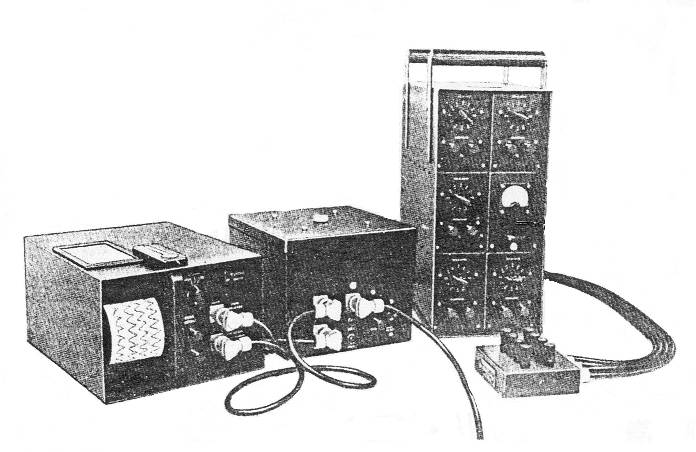
The 4 microphones were placed in shallow pits and covered with windshields (to eliminate wind noise), radio link was not used.  This recorder was primarily used for locating hostile mortars, see Counter Mortar below.

Figure 6 - Microphone
 Hot wire linear microphone as used with Recorder, SR, No 2 Mk 1

These additional elements were provided as an extra 2 sections per composite survey battery, although it did not happen all at once.  Table 1 gives a comparison of German and British equipment, it was published in March 1945.

Table 1 - German and British 4-pen Recorders
The number of sections is questionable because there were 14 British, Canadian and Indian survey regiments each potentially entitled to 4 sections, although not all were formed before the end of the war

The 4-pen recorder was one of several new devices at an advanced stage of development by 1944.  There was also a new 7 pen recorder that did not enter service.  More novel were two devices that used a cluster of close microphones to produce an accurate bearing, they did not enter service.  With the more successful, Codar, the microphones presented an oscilloscope display to provide an accurate bearing, however, it  proved insufficiently discriminatory for battlefield conditions.  

In 1945 a further enhancement was introduced, Carrier Link, SR.  This multiplexor enabled all microphones and APs to be connected to the plotting centre by a single telephone line, the transmitter units at each microphone each used a different carrier frequency.

In most cases sound-ranging was far more effective that flash-spotting in terms of the number of HBs located, although there were occasions when local conditions gave flash-spotting the edge.  However, they were complimentary because flash-spotting could be used when there was heavy firing by friendly artillery, which tended to swamp sound-ranging.  

RADAR

 In 1943 the British started mortar locating experiments with radars and in 1944 their use became quite extensive in both NW Europe and Italy. The radars used were AA No 3, Mk 2 (GL III ) and AA No 1, Mk 5 (SCR 584).  The latter were better and could produce locations accurate to about 25 yards.  The former was also used to track meteorology balloons and hence the production of meteor telegrams.  Radars designed for observing artillery fire, ground surveillance and mortar locating were advanced in development when the war ended.  However, experimental observation of fire radars were successfully deployed early in 1945 to Italy and NW Europe.  In mid 1944 British and Canadian army radar batteries were formed in NW Europe, primarily in a counter-mortar role.  The next table summarises the field artillery radars.  

 Table 2 - Field Artillery Radar Summary

 The British system of numbering radars was similar to that for wireless in that each radar role had a number.  However, there were 4 classes of radar: AA (anti-aircraft), CA (coast artillery), CD (coast defence) and FA (field artillery). Each radar role had a number within its class: AA No 3 was HAA fire control and CA No 1 was coast artillery fire control.  FA roles were as shown in the previous table.  Finally different radars with the same role number had different mark numbers.  

COUNTER-BATTERY

WW1 had taught the British that CB was best managed at corps level.  From early in WW2 each corps had a CB staff some 30 strong including seven officers, the senior (a major) being the CBO.  The doctrine was to handle CB at corps level, devolving to division level in mobile operations.  The corps CB staff could provide sections comprising an Assistant CB Officer (ACBO) and staff to two forward divisions where they worked with the HQ of a survey battery.  However, at the beginning of 1944 a third section was added and this worked with the air-photo interpretation section (APIS) in corps HQ.  This CB section had direct wireless communications with an airfield so that it could task CB sorties.  The CBO also had VHF communications to Arty/R aircraft.  The detailed organisation of a CBO staff is here.

The CB staff were provided with dedicated radio communications and were not just concerned with locating HB and attacking them.  They were also an intelligence agency responsible for CB Intelligence and providing intelligence derived from analysis of HB to the General Staff (Intelligence) branch. They used various specialist techniques to deduce information about the enemy order of battle and impending activities from the deployment and firing patterns of hostile guns and mortars.  These methods included the Shelling Plot, Hostile Battery History Sheet, Gun Density Trace, and Shelling Connectivity and Activity Trace (which showed which HBs fired where and when).  These techniques could be useful against the Germans with their short range infantry guns firing in support of their infantry regiment and small divisional artillery, because if an ARKO (artillery HQ with non-divisional artillery) appeared it was probably an indicator of an impending operation.

Data were also issued about the dimensions of German shells.  This enabled the calibre and type of shell to by determined in the field from a detailed examination of large fragments recovered from shell holes.

CB policy could be either active or passive, although in practice it was seldom this simple.  It was usually between the extremes of engaging every hostile battery that opened fire or merely locating all hostile batteries and their zones of fire so that the appropriate ones could be attacked when required.  An active policy meant attacking HB when they were located and had the goal of achieving moral and material ascendancy.  A silent policy was mostly used as a prelude to offensive operations, its premise was that it enabled a successful surprise attack on enemy batteries when and where it was needed.   The underlying assumption was that an attacked HB would move, meaning it had to be found again.  This became more complicated in the second half of the war as British artillery established their CB ascendancy and the Germans made increasing use of roving guns using temporary positions.

Deciding CB methods meant considering:

• The field defences of the HBs.
• The survey, calibration and meteorology for own batteries.
• The means and accuracy of locating HBs.
• Intelligence available about HBs' arcs of fire and habits.
• The relative numbers of target HBs and CB regiments.
• The time available.

There were standard accuracies for HB locations, the following distance 'bands' from 'truth':

• J - 10 yards
• W - 25 yards
• Z - 50 yards
• A - 100 yards
• B - 200 yards
• C - 300 yards
• D - 400 yards

A or B accuracy was the normal goal and during the second half of the war in Italy and NW Europe the survey regiments established 294 sound ranging bases and located 15,777 HBs while 360 flash spotting bases  located 4,221 HBs. at these accuracies.  A post war report pointed out that HB locating was greatly helped by the fact that Britain's enemies had not mastered multi-battery concentrations, which made locating individual HBs more difficult.

As the AGRAs evolved they had an increasingly important role and in the final stages of the war took responsibility for the CB targets in major formation fire plans with the corps CBO working from the AGRA HQ.

An HB could be destroyed or neutralized.  Destruction was best achieved by using 'pin-point' procedures with a single gun engaging a single gun with observed fire; towed guns being notoriously difficult to destroy.  However in late 1944 there was a change of tactics in NW Europe as the Germans experienced increasing difficulty in replacing their losses.  Destruction became more usual but using large amounts of ammunition, at least 100 rounds per target gun, to increase the probability of a hit.  Neutralization, in the sense of continuous suppression, was in fact a misnomer; the method of attack was short bursts of fire at irregular intervals, typically using a ratio of initially 2 to one but later 5 - 10 guns against one.   The objective was to cause casualties and damage to achieve a degree of 'neutralization' that continued after the CB fire ended.  However, this does not seem to have been notably successful because hostile batteries noticeably opened fire during lulls in CB fire.

Predicted fire was seldom really effective for CB unless there was Z accuracy, even when 'sweep and search' procedures were used to increase the size of the area shelled.  As in WW1, air observation was the best solution and Air OPs were used for observed CB fire although they often relied on seeing guns firing, and it needed luck to get the aircraft into position when HB fired only a few rounds at a time or not fire if an air OP (Auster) aircraft was in view.  However, they were also restricted in where they could fly so HBs had to be fairly close to the front for Air OPs to see them.  Sound-ranging could also range guns onto located batteries using the comparator and the ranging sections from the HQ of the survey regiment could also direct fire onto HBs using airburst ranging.

Arty/R by Tac/R aircraft was also used, because they could fly in the enemy's depth, albeit with fighter escort.  However, fighter bombers, etc were also used to attack HBs in depth and the ACBO at APIS had a direct wireless link (No 12 HP) to the Air Liaison Officer at a supporting airfield.

In NW Europe the typical CB response time from a hostile battery first firing, being located by sound-ranging or flash-spotting and CB fire dispatched was usually 12 - 15 minutes, but sometime less.  CB fire used a special type of fire plan - the 'Bombard'.  The CB staff prepared HB Lists and issued them to batteries, which produced data to engage them, excluding corrections for non-standard conditions, which were produced when the HB was engaged.  The ‘bombard’ procedure, which could be on-call or scheduled during a fire plan, or invoked any time against a troublesome HB, used the HB List.   Air observed one-on-one destruction shoots became normal, providing the terrain made the HB visible to a low flying Auster.  

Using the bombard procedure, the CB staff ordered a mix of batteries or troops to engage a listed HB using predicted fire. Aim points were distributed depending on the information available about the HB, including aiming ‘gun-on-gun’ if their co-ordinates were known. Short bursts of fire at irregular intervals were applied.  In Italy, German guns were often concealed in caves and bunkers so neutralization was ineffective.  This led to the use of Air OP observed destruction shoots. The problem was that these took a long time, perhaps only one per sortie, this in turn led to the Festa system where an Air OP engaged several protected guns simultaneously during each sortie.

COUNTER-MORTAR

After the N African campaign it was recognised that mortars were a major menace.  The problem was they were short range and deployed differently guns.  Furthermore, the existing sound ranging equipment was deployed some way behind the FDLs and had difficulty detecting mortars.  This led to new equipment and the creation of separate counter-mortar (CM) organisations as part of divisions in Italy (in about May 1944) and NW Europe.  The new organisations were independent of the survey regiments and comprised listening posts and a small control staff to co-ordinate information and arrange counter-mortar fire.   It soon became clear that similar capability was needed in NW Europe, and was formed  there.  Divisions had brigade CM sections that included listening posts and a sergeant responsible for crater analysis.  Late in 1944 divisional counter-mortar batteries were formally authorised and 13 formed for all theatres.  However, manpower constraints meant they didn't have listening posts and the theatres preferred their existing arrangements.  

New equipment development for locating HBs and mortars was well advanced in UK.   The problem was that mortars did not make as much noise as guns, the sound of a 3-inch or similar mortar firing traveled about 4000 metres and 4.2-inch 6000 metres.  This meant that a sound ranging base had to be well forward and short so that at least 4 microphones could detect a mortar firing.  The 4-pen recorder was introduced to locate mortars, its microphone base was 1200 - 1800 metres long, about 600 - 800 metres between microphones.  It had to be accepted that such a short base was not as accurate as a long one.

Four-pen recorders, SR No 2 MK 1, were trialled in Italy and Normandy in mid 1944 and selected to equip the specialist CM units.  Eventually these were equipped with both radars and 4-pen recorders and subsumed the existing ad-hoc counter-mortar organisation.  A CMO was created at divisional HQ and worked with the ACBO as part of HQRA and there was an ACMO at each brigade HQ, often an infantry officer.  

Airborne divisions also received a CM capability by adding listening posts, 2 × 4-pen recorder sections and a plotting centre to the Forward Observation Unit (Airborne).

Nebelwerfers didn’t fit neatly into either CB or CM and one or other would take responsibility by local agreement.   

Counter-mortar shoots were a different proposition to guns because mortars, being small with few vulnerable parts, were even more difficult to destroy.  The aim was to cause casualties to the mortar crews.  This required a quick response when a mortar was located so CM officers were often assigned a battery.  CM fire usually used airburst HE or other mortars, particularly 4.2-inch when they were available.  The 3.7-inch HAA was popular for the first because of its effective airburst fuzes but 7.2-inch How was also widely used.

AFTER WORLD WAR 2

At the beginning of 1948 survey regiments and batteries were re-designated ‘Observation’ and then in the early 1950's 'Locating’.  Shortly after the war regiments were re-organised back into specialist batteries (survey, observation (ie flash spotting), sound ranging and radar (both ground surveillance and mortar locating)).  For the decade following the war there was little other change.  Flash-spotting continued to refine its methods (including the method for locating rocket launchers) and minor changes to equipment.  However, its relevance and capability was declining as ranges increased and flashless propellant became pervasive, and its continuation was probably mainly  for airburst ranging.   The FS capability was finally suspended  in about 1961, although it was still taught on Gunnery Staff courses for several years after this.  Sound-ranging reverted to line communications only, probably due to radio link's inability to give the APs remote switch on/off, the unsuitability of radios for unattended operation and the introduction of Carrier Link, SR, that significantly reduced the amount of cable laying and maintenance.  A new sound-ranging Recorder No 5 was introduced, this used Teledeltos paper with 7 'pens'.  Various radar developments continued.  At the end of WW2 counter-battery and counter-mortar were combined and called counter-bombardment.  In the late 1950's counter-bombardment staff were renamed 'artillery intelligence', although there was no change in responsibilities and the staffs had become part of HQsRA at division and corps instead of being organisationally separate.  The new artillery control term 'at priority call' was primarily intended for counter-battery use.  In 1960 full responsibility for artillery meteorological data was at last transferred from RAF to RA locating.

A CB staff and observation battery joined the Commonwealth Division in Korea, the battery having sound-ranging and two FA No1 Mk 1 counter-mortar radars, which had finally entered service but were not very successful.  Subsequently AA No 3, Mk 7 (F) was used, this had entered service shortly after WW2 and had auto-tracking.  However, an important innovation was the provision of counter-mortar staffs to the tactical HQs of  direct support field regiments.  An ad-hoc locating ('Cracker') battery comprising sound-ranging and mortar locating radars were deployed in Borneo, and radars in South Arabia in the mid-1960's.  Mortar locating radars and sound-ranging were also deployed in Oman in the early 1970's.

In about 1960 target acquisition capability advanced significantly with the introduction of new equipment. An excellent mortar locating radar (FA No 8, Green Archer), with a silenced generator was introduced.  This used a Foster scanner that produced a very narrow beam angle and spread its pulses horizontally to give very wide but vertically  narrow, beam, with the antenna having two mechanically fixed positions that the operator switched between.  This produced two positions for a mortar bomb in flight and since a mortar trajectory is close to parabolic it was very simple to calculate the base plate position from these two points.  This eliminated the need to track the bomb, a significant weakness in the earlier generation of equipment.  FA No 8 was replaced in the mid-1970's by another radar with a Foster scanner, FA No 15 Cymbeline, although in this case the beam was switched electronically between horns not mechanically moving the antenna.  

The introduction of FA No 8 led to the de-centralisation of mortar locating, a troop of two radars and an artillery intelligence section was added to each direct support field regiment reflecting the lessons of WW2.  Divisional survey troops became part of divisional nuclear artillery regiments.  This left space to add new capability alongside sound-ranging and new meteorological troops.

Also in about 1960 a long range ground surveillance radar (GS No 9, Robert) mounted in a Saracen APC was introduced, it lasted about 10 years.  It was not replaced, the British having decided that long range ground surveillance radars had limited utility.  Instead they adopted short range radars for every artillery observation post, although the second generation of such radars introduced in 1990 had longer range that Robert!  

More significantly an unmanned aircraft the SD-1 drone was introduced at about the same time, perhaps reflecting the conversion of AOP to Army Air Corps and realisation that tactical air reconnaissance was likely to be less available.  This unmanned aircraft was capable of wet film photography by day or night.   It was radio controlled from the ground with the controller watching a continuous plot against a paper map displayed in a FA No 13 radar.  It too lasted about 10 years and was replaced by a true drone (ie flying a pre-programmed course), AN/USD 501 Midge (also known as CL89), which had its only operational outing in the 1991 Gulf War, subsequently being replaced by Phoenix.  This all makes the Royal Artillery the longest continuous user of battlefield UAVs, although it took some 40 years for the rest of the Army to waken to their potential!

Late in the 1960's effective radio-link sound-ranging was introduced, it enabled the APs to switch on the recorder and line finally abandoned.  A few years later the advent of programmable electronic desktop calculators meant that manual plotting could also be replaced. The same calculator was vast improvement over the mechanical calculators, such as Brunsviga, used for survey calculations.  However, the big change in the 1990's was again led by the British adopting a new approach to sound-ranging, new technology made the CODAR approach viable.  The microphone base was replaced by several unattended microphone clusters, each cluster had a computer, microphones and meteor sensors, and it produced an accurate bearing to the HB.   This and other data were sent automatically to a plotting centre where they were automatically collated to produce the HB location and further analysed.  This prototype system, HALO, performed well in the Balkans and was subsequently replaced by an even more sophisticated one that was used in Iraq in 2003, reportedly locating Iraqi batteries at over 50km distance.

 Copyright © 2002 - 2014 Nigel F Evans. All Rights Reserved.