INTRODUCTION

This page gives an outline of ballistics as applied to artillery.  It explains the influences on a shell in flight and the variations that they cause, the factors affecting muzzle velocity and the data in and evolution of range tables that enabled corrections for these variations.

Ballistics is the applied science of the motion of projectiles.  For artillery there are probably at least three significant perspectives, those of:

•    the theoretician,

•    the gun and ammunition designers, and

•    its practical application by artillery in the field to predict the trajectory needed to hit a target.  

The last of these involves developing methods that can be used in the field to aim guns and correct for variations in ballistic conditions.  It involves instruments, ‘base data’ and ‘data of the moment’ and the procedures for combining them.  This site focuses on artillery and hence the practical application of ballistics so this page focuses on the third perspective.

Military ballistics is usually divided into internal, intermediate, external and terminal ballistics.  Intermediate ballistics is what happens as the projectile leaves the muzzle, terminal ballistics with the effects of the projectile or its pieces on the target.  External ballistic variations are the main concern for artillery in the field and this page is mainly concerned with external ballistics.  Internal ballistics is also vital but, apart from charge temperature and variability in ammunition, sustained variations occur relatively slowly.  The major aspect of internal ballistics that affects practical gunnery is variation in muzzle velocity (MV).  This changes over long and short terms and is dealt with on the Calibration page together with aspects of internal ballistics.  Atmospheric data are dealt with in Meteor.  Aspects of terminal ballistics are described in Effects and Weight of Fire.

BALLISTICS OF A SHELL

Trajectory

The basics of external ballistics are simple, if a projectile is fired in a vacuum affected by gravity at some angle of elevation then it will follow a parabolic trajectory to hit the ground.  The constant curve is the result of gravity.  However, the earth has an atmosphere so the projectile is slowed by air resistance.  This significantly reduces the distance (or ‘range’) that the projectile travels before hitting the ground.  For a rifle bullet the range loss may be as much as a factor of 20, for an artillery shell perhaps a factor of 3 or 4 depending on its calibre.  Air resistance also means the trajectory fired at an elevation of less than 45° is no longer parabolic, but elliptic - a segment of an oval curve:

• its highest point (vertex) is no longer mid-way but closer to the target,
• the angle of descent is steeper than the angle of departure, and
• the impact velocity is less than the muzzle .  

An implication of this oval segment trajectory is that, without any angle of sight,  maximum range for any charge is given by an elevation angle of about 45°, however, 50% this elevation angle gives about 80% of maximum range.   A shell loses velocity along its trajectory, although it gains a little in the final 10% or so of maximum range when the angle of descent steepens significantly and gravity makes a noticeable contribution.

Gravity also varies slightly and the total effect depends on and is a major determinant of the shell's time of flight because the total effect depends on the exposure time to the gravitational force.

Figure 1 - A Shell's Trajectory

Air resistance is not a simple factor, it affects a projectile in several ways and is not a constant.  Air behaves as a fluid, it is actually denser than water vapour, has higher viscosity than water or water vapour, and its viscosity changes with atmospheric conditions.  Air resistance affects a projectile in flight by causing:

• Skin drag, air friction on the projectile.
• Pressure drag, caused by pressure differences between the front and rear of the projectile, however, there are important differences between sub- and supersonic speeds and these make transonic speeds particularly problematic.
• Yaw drag, arises from differences between the tangent of the trajectory and the long axis of the projectile, it is a function of the projectile’s stability.

Air resistance varies throughout a shell's trajectory and with continuously changing meteorological conditions, it is also affected by the shell's ballistic shape.  The total effect of air resistance depends of the trajectory length because that determines the amount of air resistance to be overcome.

While the basic theories were understood from the late 19^th Century, measuring or estimating actual drag and developing equations of motion that accurately apply the various and variable effects to projectiles of various shapes and sizes was a complicated matter that evolved over many decades.  Obviously improvements in instrumentation were a significant factor.  In the 19^th Century key work on measuring air resistance was by the Rev Francis Bashforth who was the professor of applied mathematics to the artillery advanced course at Woolwich.

A projectile also has to be stable in flight, this means that the long axis of a shell is close to parallel to the tangent of the trajectory throughout the trajectory.  For artillery shells this stability is produced by spinning the projectile to produce the gyroscopic effect - keeping the axis of spin stable.  The smaller the projectile the faster the rate of spin to stabilise it.  For artillery projectiles spin rates in the order of 20,000 revolutions per minute are needed, rifle bullets are an order of magnitude greater.  Spin is created by rifled barrels engaging the driving band(s) of the shell.  The rate of spin is determined by projectile velocity and the pitch of the rifling.  The alternative to spin is fins, this achieves stability by ensuring the centre of pressure is well behind the projectile's centre of gravity.

A spinning shell can be over-stable, this means its axis remains parallel to its angle of departure from the barrel and it lands base first.  Of course the rate of spin also changes with a shell's remaining velocity throughout its trajectory.  Furthermore the ideal rate of spin varies with the angle of the tangent of the trajectory to the horizontal plane and with projectile length.  

The combined effects of air resistance can be reduced to a drag co-efficient for a shell.  This co-efficient is widely used to represent a projectile’s aerodynamic efficiency.  It has the form C_D=8(Drag Force)/ρV²πi.d² where ρ = fluid density, V = velocity in flight and d = projectile calibre, in practice d becomes the frontal area and 2 is included in the numerator.  In practical terms the drag co-efficient is a function of velocity, usually represented as the Mach number that varies with air temperature, which in turn reduces with altitude.  The drag co-efficient is estimated during ammunition design, or since computer simulations became possible, it can be modeled.  These estimates can then be confirmed or adjusted from ‘range & accuracy’ firing during development.

Another widely used data is the ballistic co-efficient.  This reflects the rate at which velocity is lost as the projectile penetrates air.  The ballistic co-efficient is sometimes called the ‘carrying power’ of a shell, meaning how far a given muzzle velocity will ‘carry’ it.  It is expressed as C_B=M/nd², where C = Carrying Power, M = projectile mass, d = projectile diameter and n = κστ, where κ (kappa) is the co-efficient of shape, σ (sigma) the co-efficient of steadiness and τ (tau) the co-efficient of air density.

This means that mass is the main determinant of carrying power and is the reason that artillery shells go further than rifle bullets even when the latter are fired at higher velocities.   For a particular muzzle velocity and firing elevation angle the heavier shell will always go further (unless its shape and steadiness are significantly inferior).

Of course the parameters and co-efficients are not constant.  The Drag Co-efficient varies with projectile velocity.  Particularly important, the density of the atmosphere varies with altitude.  In flight, a projectile's velocity decreases with gravity and air resistance until vertex is reached, when air resistance continues but gravity accelerates the projectile as it descends (hence the elliptic trajectory).  The rate of spin (revolutions per second) also decreases with velocity throughout the shell’s flight, which affects its stability.  Gravity is not constant either, it decreases with distance from the earth’s surface (which is uneven).  Furthermore the atmosphere itself changes continuously with atmospheric conditions, this is explained on the Meteor page.  

Until about the 1950s it was thought that to ensure steadiness the shell calibre to length ratio should be between about 1:3.5 and 1:4.5, and this is reflected in WW2 shell designs.  However,  longer shells subsequently proved possible and have become normal.   One element of the shape co-efficient  is streamlining.  Increasing velocity requires a more streamlined shell shape, the curvature of the shell's nose or 'ogive', which was defined by a ratio called the 'circular radius  head' (crh) .   This streamlining started in WW1.  The need for a streamlined shape becomes greater with increasing velocity because of the changing shape of the pressure wave formed as the projectile nose cleaves the atmosphere.  

There are other factors that affect a projectile in flight in addition to air resistance and gravity:

• Wind, with head/tail and left/right components depending on the wind speed and the relationship between the wind direction and the line of fire.  Wind varies throughout the trajectory in terms of its speed and direction and the total effect depends on the time of flight exposure time.
• Equilibrium Yaw, has three consequences: yaw drag (above); it causes a projectile to move to the side, called drift in gunnery; and it provides some lift, which increases range.  Yaw is the consequence of spinning the projectile.
• Rotation of the earth, only significant at longer ranges, there are three factors involved so the size of correction varies with latitude and bearing of fire.  It affects both range and line.  It is not large, typically at 10 km range and 50° Latitude range corrections vary between zero and 25 metres and line (left or right of the line of fire) between 15 and 25 metres on the ground at the target.  It is greatest at the equator because this is furthest from the Earth's axis.

Drift is the term given to a projectile's tendency to deviate from its trajectory and is caused by the projectile spinning.  In British guns, which have clockwise rifling (viewed from behind the gun), it is to the right and is the nett result of several influences.  Equilibrium Yaw tries to pull a shell upwards but the gyroscopic effect reacts to this by moving the shell in the direction that its topside is spinning, to the right.  This is much stronger than the Magnus effect that forces the shell to the left, which in turn is stronger than the Poisson effect forcing it rightwards.

Muzzle Velocity

The distance that a shell travels is a function of its muzzle velocity, angle of projection at the muzzle, projectile mass and the external ballistic characteristics and influences.  This means that internal ballistics cannot be ignored because they determine the muzzle velocity, which varies for several reasons:

• Propellant energy, determined by quantity and type, multi-charge guns (technically howitzers) have charges of different weights that give different ranges for the same angle of projection.
• Projectile weight, different types of projectile have different weights.  Manufacturing tolerances mean that different production batches may differ slightly in weight.  Different fuzes can also differ in weight due either different functions or different materials, such brass or aluminium bodies.  A heavier projectile fired with the same amount of propellant will have a lower muzzle velocity than a lighter one.
• Propellant temperature, which causes variations in energy, the gunnery significance is that temperature varies in the field, typically a change in propellant temperature of 10°F changes muzzle velocity by 0.5%.
• Barrel wear, which generally means that a barrel’s muzzle velocity reduces with the total number of shells it fires.  Broadly, it is generally agreed that a barrel should not be used when its physical wear reaches about 3% of calibre, which represents about 5% loss of muzzle velocity.

Muzzle velocity also varies slightly round to round, this is explained on the Calibration page.  Given basic data and data about the variations from standard conditions then corrections can be calculated.  However there are residual variations, most reflected in round to round variations in muzzle velocity that underlie range Probable Error.  

Other Factors

The gun itself also affects the projectile’s flight.  The axis of the bore at the breech may differ slightly from the axis of the bore at the muzzle, this is called ‘droop’.  Furthermore the movement of the projectile may cause some ‘whip-action’, which means the axis of the bore at the muzzle (in the vertical plane) when the projectile leaves it is different to its axis before firing.  This is called ‘jump’.  Traditionally these were both given constant values for a charge, although in reality they are means with small variations.  Jump can originate in both the barrel and in elements of the carriage or mounting.  For example with 25-pdr at charge super, the Mk 1 Carriage (ie '18/25-pdr') had 27 minutes of jump while the Mk 2, the 'proper' carriage only 7 minutes. Jump is usually presented as vertical and upwards, but may have horizontal components as well although before modern trials instrumentation this was probably measured in drift.

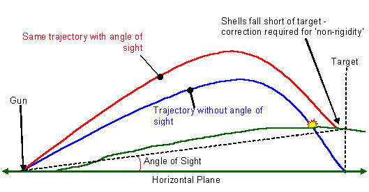
Finally, a difference in height between a gun and its target also affects the trajectory.  Therefore, the angle of sight has to be added to or subtracted from the gun’s firing elevation angle.  However, the slant range to the target is greater than the horizontal range and applying the angle of sight does not compensate for this, which is called non-rigidity of the trajectory.  The size of the correction for this depends on the difference in height between the target and the gun, and the shell’s angle of descent.  This angle is in turn determined by the gun’s muzzle velocity and the range to the target.  Furthermore, altering the elevation angle also puts the trajectory through a different ‘slice’ of the atmosphere, where air resistance may be different.

Figure 2 - Non-rigidity of the Trajectory

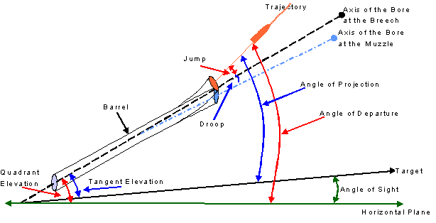
This leads to the subject of ‘Ballistic Angles’, or perhaps more correctly 'Gunnery Angles',  the various elevation angles related to a barrel and a shell fired from it.  No page referring to artillery ballistics is complete without this illustration, tradition demands it.  At the other end of the trajectory the Angle of Descent is the angle at the point of impact between the line of sight and the tangent of the trajectory.

Figure 3 - Ballistic Angles

Jump and Droop are extremely exaggerated in size

Data and Calculations

The heart of the ballistic problem for practical gunnery is to determine the muzzle velocity and angle of projection that are needed to give the distance for a projectile to hit its target.  There are only a small number of choices for muzzle velocity (the number of different charges available for the gun).  Closely related but somewhat simpler is the need to determine the horizontal direction.  Combining these to predict the required trajectory is the challenge.  Both distance and direction can be measured from a map or calculated from co-ordinates but distance then has to be converted to an elevation angle and both have to be corrected for ballistic variables.  

Understanding ballistic theory is one thing, applying it in the field to predict a required trajectory is a different matter altogether.  The first step is a mathematical model, a set of equations of motion, to describe a projectile’s trajectory and allow the variables to be represented.  From the late 19^th Century onwards many models were developed and refined.  They also had to be solvable by available mathematical techniques, and most importantly be usable in the field.  Given the complexities and uncertainties involved, combined with difficulties in getting accurate data, these models and their data contained many approximations and simplifications.  The second step is to derive methods and data from these models that can be used in the field.

In the first years of the 20^th Century numerate artillerymen, basically the Royal Garrison Artillery as far as UK was concerned, could adjust the ballistic co-efficient to correct for local conditions.  They used methods detailed in the Text Book of Gunnery and associated data tables.  From 1897 Table VII of the Text Book provided the Rev Bashforth’s Tenuity Table, which had been published in the Journal of the Royal Artillery in 1886.  This table gave factors for barometric pressure in inches against air temperature in degrees Fahrenheit, based of standard conditions of 30 inches and 60°F, and allowed tau to be adjusted.  The 1911 edition of the Text Book Part 2 also provided a nomogram derived from Bashforth’s table that gave a percentage alteration in the ballistic co-efficient for variations in air temperature and pressure.  The 1914 edition of Part 1 went further with a table of relative densities (tau) which divided Bashforth’s data by 534.2 (the weight in grains of a cubic foot of standard air) and then adjusted it to reflect a loss of 1 inch pressure per 1000 feet and 1°F per 300 feet of height (the adiabatic lapse rate).  It also explained that data should be used for a height at 2/3 expected vertex (maximum height of trajectory).  Trajectory vertex in feet could be deduced using the simple equation 4T², where T was time of flight (given in Range Tables).  However, in World War 1 (WW1) it quickly became clear that better methods were needed.  This led to extending the data provided in Range Tables.

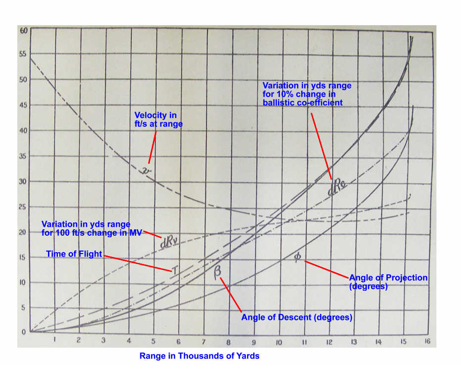
During 1904-06 UK had conducted experiments to re-define air resistance (and this was again undertaken in the 1920's).  Producing Range Tables meant that more data had to be extracted from range & accuracy firings.  This process involved firing several series of shells at different elevations, plotting their impact with great accuracy, and recording data about environmental conditions, MV and jump.  Analysis of this data led to calculations of different components.  First the 'primary variations', which in turn enabled calculation of the secondary variations.  Figure 4 shows the primary variations for 60-pdr.

Figure 4 - Primary Variations

The starting point was an estimated ballistic co-efficient and assumed shape (κ kappa) and steadiness (σ sigma), and then refining κσ to fit the observed data.  The calculations were simplified by extensive data tables for various ballistic functions.  Once κσ had been ‘fixed’ it was graphed with elevations between 0° and 45° (or whatever the maximum elevation was) on the horizontal axis.  Then a set of very large graphs were prepared for standard elevations at standard conditions using κσ and data from tables of ballistic functions, and from these were read range table data for every 100 yards.  This method lasted into the 1950's.

Calculating data for range tables was an early use of electronic computers.  This led to new models that combined the relevant and most important equations of motion in computationally efficient ways.  The simplest was the Point Mass Model.  This treated a projectile as a point with ballistic co-efficients moving with 3 Degrees of Freedom (two horizontal and one vertical).  However, while this was satisfactory for some purposes it was not entirely satisfactory for artillery where projectile yaw is a major consideration.  This led to the Modified Point Mass Model with 4 Degrees of Freedom.  As computing power increased and computers shrunk it became possible to process these models in field computers.  

The most accurate model uses 6 Degrees of Freedom (pitch and roll are included).  However, this requires a lot more computational power (or time), does not give a significantly better solution for guns and requires ‘start state’ data that is difficult to provide.  Its use is generally limited to ammunition design and with rockets.

However, some handheld electronic calculators, introduced in the 1970's and 80's for 'back-up' calculations took a different approach.  They in essence replicated the manual methods, but used polynomials to represent the tabulated data provided in firing tables.  

RANGE TABLES

Range Tables (RTs) detailed the performance of a gun under standard conditions and dealt with both internal and external ballistics.  Tables that related elevation and the amount of propellant to range had been used for centuries, for example those produeced at Dover Castle by Master Gunner William Eldred in 1613.  Before WW1 they had some additional data, but during WW1 the content of RTs increased dramatically to meet the needs of ‘map shooting’.  They were enhanced to provide data to convert variations from standard conditions into corrections to the range and azimuth set on the guns’ sights.  Generally there was one RT for each combination of type of gun and ammunition ‘family’.  RTs lasted until NATO standardised Tabular Firing Tables (STANAG 4119) were introduced in the early 1970's.

RTs were published before 1914 for all guns and howitzers.  However, compared to later editions their content was sparse.  The main table for a charge provided data at each 100 yards of range:

• Elevation angle.
• Shrapnel fuze length.
• Angle of descent.
• Remaining velocity.
• Time of flight.
• The values in yards of 5 minutes elevation and deflection.
• Deflection for drift.
• ‘Accuracy’ (actually ‘consistency’) as the 50% zone.

The first two items converted distance into firing data and Drift data provided a correction to the azimuth.

The data given in these RTs was for ‘standard conditions’.  These were defined as no wind, barometric pressure 30 inches of Mercury and air and propellant temperature 60° Fahrenheit.  They remained British standard conditions until the mid-1950's, albeit with refined definitions.  However, in 1915 RTs started changing from their pre-war simplicity by including data for  variations from standard conditions.  The first appears to have been for the 9.2-inch howitzer in the second quarter of 1915, although it seems to have taken another 12 months or so to issue them for most guns and howitzers.  The data in these ‘modern’ RTs was used to calculate corrections to range and deflections to the angle from the Zero Line.

Initially, in 1915, two approaches were used.  A few RTs provided alterations in range for a change in MV and for wind along the line of fire and Correction Cards were issued for other guns.  The latter seem to have only covered wind, barometer and air temperature on the lines proposed just before the war.  

The Correction Card for 18-pdr was complicated by the change in shell shape brought about by the introduction of HE with a new matching Mk 2 shrapnel shell, which affected the ballistic co-efficient, and a RT MV that was not representative.  This meant that the range indicator, a disk with a range scale fitted to the guns and giving the relationship between range and elevation angle (range not elevation angle was ordered to the guns) for the Mk 1 shell was no longer valid.  The Correction Card used the temperature correction to provide a single range correction figure at each range for the newer shell, revised MV, air and charge temperature (assumed to be the same value, but in practice usually not).  This approach was not used in RTs where separate data was given for each variable.  

From mid 1916 RTs provided variation data for all the standard conditions. Initially the main table was unchanged and additional tables were added for each type of variation.  By late 1916 the separate variation tables for each charge were consolidated into one table per charge, starting with the highest charge.  They provided variations in yards, tabulated for each charge at every 500 yards of map range, for variations from non-standard conditions.  The pre-war standard conditions, no wind, 30 inches of Mercury air pressure, and 60°F air and propellant temperature, were unchanged.  The data were provided for:

• 100 ft/sec decrease in MV.
• Change of 1 inch in barometric pressure.
• Change of 10°F in air temperature.
• Change of 10°F in charge temperature for each type of propellant.
• 30 ft/sec following wind.
• 30 ft/sec cross wind.

These data were used to calculate corrections.  For example if the effect of a variation of  +1 inch pressure was to reduce range by 100 yards, then if the actual pressure was 29.5 inches  the correction was -50 yards.

However, a modification of the Correction Card approach continued to be used.  While care had been taken to ballistically match HE and Shrapnel so that they used the same data new ammunition was appearing.  Chemical, Incendiary, Star and Smoke couldn’t be matched and had different ballistic co-efficients.  Separate tables were issued, initially called ‘Range, Elevation and Fuze Scales’.  For map range these gave the non-standard elevation, fuze length and time of flight.  In the last year of WW1 these became Supplementary Range Tables, either as separate documents or appendices in the main one.  For guns with a range indicator a ‘false range’ was added, this converted the range for the non-standard shell into the equivalent range for a standard shell.  This range was set on the range indicator.

By 1918 the general structure of RTs was a table of contents and introductory notes, a section for each charge, and additional notes or appendices at the back.  Data for each charge started with details of standard propellant, MV and projectiles, then a main data table with many columns, typically about 20 extending across both pages, then various other tables and graphs.  However, guns (ie supposedly a single charge) were slightly different, data for their reduced charge was provided in a separate RT.  Separate RTs were also provided for shells with different crh (ie ogive shape).  At the start of the war 1½ crh had been normal, by the end 60-pdr had reached 8 crh.

By the end of the war the data had increased to include, as applicable, variations arising from different fuze types, shell weights (per ½ lb increase for smaller calibres), different models of driving band and 10% variation in ballistic co-efficient.  Drift was still included, although in some guns this was incorporated in the sights, as was jump.  Some of these were in the main tables others either a single figure per charge or separate tables.  Also included were wind correction tables that enabled range and deflection correction to be calculated for different elevation angles (every 10°) and ranges (every 1,000 yards) between the wind direction and line of fire per 30 or 100 ft/sec of wind depending on the gun.  

By this time most data were expressed as corrections, mostly for a variation that was a decrease, ie corrections were the variation with the sign reversed.  In other words, using the example above,  where the effect of a variation of  +1 inch pressure was to reduce range by 100 yards, then the tables now gave the actual correction to be made, +100 yards in this case.  However, it wasn't quite that simple because the necessary correction value is not the same as the variation.  For example if a head wind causes the shell to be 200 yards short, then adding 200 won't be enough because the head wind is also acting on the extra 200 yards causing it to be a bit short.  The correction actually has to be [(range/range+variation)*variation], so if a variation is negative the positive correction is slightly greater in value that the variation with its sign reversed.

Addenda, called amendments from the 1920's, were also issued.  They included new pages, manuscript changes or ‘cut and paste’ insertions.  These ranged in scope from a single column in a table or paragraph of notes to substitute pages.  Some early RTs had many addenda and in many cases the WW1 tables themselves were replaced by a new edition within a year during the war.  This reflected the rapid pace of their evolution and the introduction of new ammunition.

In 1920 Artillery Training Volume 2 – Gunnery (Provisional) appeared and replaced all the various gunnery publications.  It listed the sources of variations that affected line, range and corrector (for airburst fuze setting) as follows:

The underlined variables were those that changed rapidly and ‘normally taken into account’.  Muzzle Velocity (MV) was adjusted in accordance with calibration results.  Charge temperature and projectile variables also alter MV, however, in RTs these and MV itself were usually treated as corrections to range.  Drift was provided in RTs as was Jump and Droop.  However, it was also British practice was to accommodate Jump and Droop in the sights unless they varied with charges (jump usually did, droop didn’t) and some guns had a drift scale as part of the sights.  

The notable omission is Rotation of the Earth (RoE).  In 1915 the Navy had raised the issue and been advised that it was included in the Drift correction.  Of course correction for RoE reflects both azimuth and range variations and its size depends on latitude and the azimuth of the line of fire relative to the equator.  No doubt the line correction for Shoeburyness, on the N Sea coast, incorporated into Drift was helpful for the Grand Fleet and its N Sea operations.  It’s unclear if and when RoE was removed from Drift in artillery RTs.  However, RoE did not start specifically appearing in RTs until the 1950's.  By this time fuze weight had ceased to be an issue as had the possibility of different driving bands for a shell.

The Text Book of Ballistics and Gunnery 1927 included details of the standard structure and content of RTs, although these seem to have stabilised by the early 1920's.  The standard MVs used in range tables were that estimated for the gun when it was a quarter worn.  The body of the tables provided data for every 100 yards of range with the associated TE or Angle of Projection, drift, time of flight, 50% zones, minutes elevation for 100 yards on the ground, and subtension angles for 100 yards lateral and 100 ft vertical at graze.  Also in the main body table for each charge were corrections for variations of:

• MV (at + 50 and – 50, 100 & 150 ft/sec).
• Change of 1 inch in barometric pressure.
• Change of 10°F in air temperature.
• Change of 10°F in charge temperature for each type of propellant.
• Projectile weight difference (units (lbs) depended on the shell weight).

The different corrections for MV reflect the fact that variations can be non-linear.

Separate tables provided:

• Table of range corrections (yards) for 10 ft/sec of wind at every 10° angle between wind direction and azimuth of fire in the range 0° to 90° and a similar table for deflection corrections in minutes.  Alternatively, these data could be presented graphically in a chart.
• Non-rigidity table.
• Angle of descent table.
• Drift tables, if drift was not in the main body table.
• Data for fuzes including corrector corrections for variations.

A revised Text Book of Ballistics and Gunnery appeared in 1938.  It changed RTs by adding Calibration Data and Crest Clearance tables.  An amendment in 1942 changed most of the subsidiary tables.  In both cases the Text Book was documenting changes that had already been made:

• The chart (a wind resolution graph) became the standard means of providing wind corrections.
• Non-rigidity was provided both as a table and a chart.
• A separate table (data every 500 yards) was provided for Angle of Descent, residual velocity, range correction for 1% change in ballistic co-efficient and drift.
• Tables and data for calibration (corrections to range for variation in MV and variations in MV for wear).
• Crest Clearance table.
• Chart of non-rigidity corrections for use with airburst ranging.
• Fuze corrections for abnormal conditions.

A simplified calculation for meteorological corrections was introduced in 1944, it required appropriate data (‘Taylor Tables’) in RTs.  These gave, for each charge, correction to range (and line for cross wind) for the values given in the met message against the time of flight ‘band’ (10, 20, 30 secs, etc).  This was in addition to the conventional data given in the main table for each charge.  At much the same time new tables were introduced giving variations in MV, for different propellant types and measured barrel wear so that guns’ MVs could be updated from wear measurements, see Calibration page.

The format of RTs changed again in the 1950's, mainly to add data to that that had been provided by the end of WW2.  By this time another issue was considered relevant – cross-term effects.  Prior to this corrections were on the basis that variations were independent of each other.  This was generally reasonable but could cause errors at extremes.  One example that was accommodated in new RTs was Non-rigidity and MV, Non-rigidity reflects the Angle of Descent, which changes with MV as well as range.  New Non-rigidity graphs were read at both range and MV, there were graphs for both low and high angle, and graphs of corrections (used during prediction) and variations (used for reduction of firing data to calculate target co-ordinates).

The other changes during the 1950's included:

• introduction of colour coded page tabs for each charge (colours being those of the charge bags themselves when these were differently coloured),
• a graph to select the Met Line Number for the charge, range and angle of sight (this was necessitated by introduction of the NATO Ballistic Met Message),
• inclusion of Rotation of the Earth (RoE) data, although this did not appear quickly,
• correction for the differences between the UK and ICAO standard atmospheres,
• auxiliary barometer table for use with a large change in ballistic co-efficient.

The last two were both for use during calibration.  In addition, in the late 1950's NATO agreed to standard units of measurement, none of which had been used by UK.  Existing instruments and RTs were converted or replaced in the following 10 years.

In the late 1960's NATO STANAG 4119 Standard Firing Table Format was agreed.  This ended RTs.  Tabular Firing Tables (TFT) were not a total novelty to UK because the US Firing Tables had been used with the US guns introduced in the 1960's (and 20 years earlier in WW2 before RTs for US guns were available).  The first TFT for UK guns was that for 105-mm L13 Abbot, which replaced its RTs in 1971.  The STANAG also covered Graphical Firing Tables (GFT), these had not previously been officially adopted by UK, although similar devices had been produced by entrepreneurial officers during WW1 and the Battery Rule of that period had a similar function as did the Rule, Correction, BC of about 1940.  

TFTs contained true corrections and not merely variations with the mathematical sign reversed.  The other significant changes were the introduction of density data instead of barometric pressure and changing the standard charge temperature from 60°F to 21°C (70°F), which increased the standard muzzle velocity and had the effect of slightly increasing the maximum range for British guns.  However, by the time TFTs were introduced a digital computer was in service and TFTs were used only for back-up.  The structure of TFTs is:

• Introduction providing common data about the gun and ammunition.
• Part 1, comprising ‘chapters’ for each charge number, with data in standard format tables A to K.  The Basic Data table, F, is split into two sub-tables.
• Part 2, provided data for non-standard ammunition.
• Appendices provided additional data for such matters as Crest Clearance, Calibration, and Trajectory Charts.
• Supplementary volumes provided any data for national procedures.

In the same period there were other agreements, notably AOP-1 Ballistic Standardization of Gun Ammunition and STANAG 4115 Definition and Determination of the Ballistic Properties of Gun Propellants.  The goal of this was ballistic standardisation so that guns of one nation could fire ammunition produced in another.  Partial standardisation meant this could be done safely and full standardisation meant it could be done without recourse to special fire control data.  Several other STANAGs relating to ballistic matters were also created.

WAR OFFICE PUBLICATIONS

Text Book of Gunnery, Capt G Mackinley RA, 1883.

Text Book of Gunnery, 1887.

Text Book of Gunnery, (3rd Edn), Parts 1 and 2 (mathematics) in a single volume, 1896.

Text Book of Gunnery, Part 2, 1911.

Text Book of Gunnery, Part 1, 1914.

Hand Book of Ballistics, Vol 1, External Ballistics, C Cranz & K Becke, translation of German 2nd Edn, 1921.

Textbook of Ballistics and Gunnery, Part 1, 1927.

Textbook of Ballistics and Gunnery, Part 1, 1938, reprinted 1942.

Textbook of Ballistics and Gunnery, Part 2, Sect 3, Theoretical Principles of Gun Construction, 1933 reprinted 1941.

Textbook of Ballistics and Gunnery, Part 1, Definitions, Motion in Vacuo and Laws of Air Resistance, 1948.

Textbook of Ballistics and Gunnery, Part 2, Siacci Equations, Primary and Secondary Ballistic Functions, 1954.

Textbook of Ballistics and Gunnery, Part 3, Stability and Drift, 1951.

Textbook of Ballistics and Gunnery, Part  4, Meteorology and Meteorological Constraints, 1952.

Textbook of Ballistics and Gunnery, Part  6, Construction of Range Tables, 1954.

Textbook of Ballistics and Gunnery, Part  8, Sighting, 1946.

Textbook of Ballistics and Gunnery, Part  9, Dispersion of Fire, 1947.

Textbook of Ballistics and Gunnery, Vol 2, ed LW Longdon, 1984.

Textbook of Ballistics and Gunnery, Vol 1, 1987.

Artillery Training (AT)

AT Vol 2 Gunnery, Chap 1 Ballistics,1928.

AT Vol 2 Gunnery, Chap 1 Ballistics,1934.

AT Vol 3 Pam 1 Ballistics and Ammunition, 1948.

AT Vol 3 Pam 1B Ballistics and Technical Aspects of Field Gunnery, 1959.

Unofficial publications

Guns, Shells and Rockets - a simple guide to ballistics, Major JCS Hyman, 1950.

Military Ballistics - A basic manual, GM Moss, DW Leeining, CL Farrar, Brassey's Land Warfare, 1995.

 Copyright © 2006 - 2014 Nigel F Evans. All Rights Reserved.